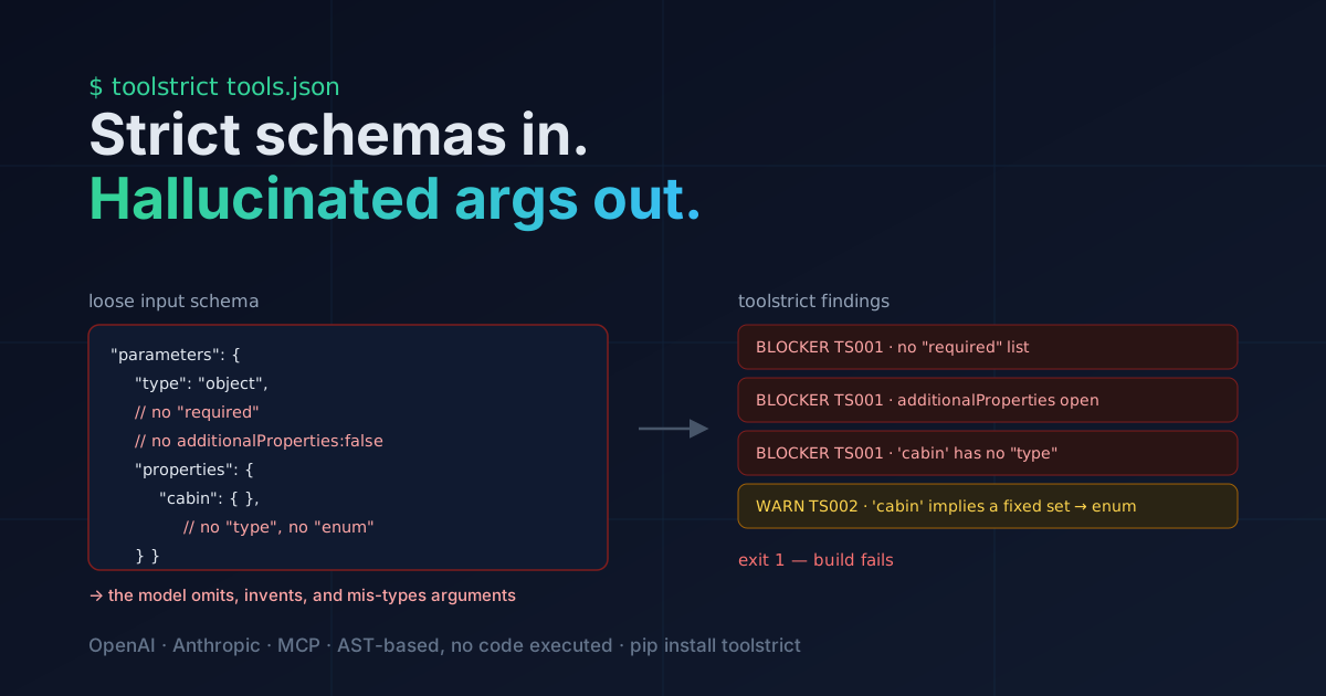
Your cloud bill knows the dollars, not the carbon. cinderscope estimates the kgCO2e - offline.

Finance has known the shape of your cloud spend for years: an invoice, a cost explorer, a dozen FinOps tools that slice the dollars by service, team and tag. Ask the same stack a different question - how much carbon did that run? - and it goes quiet.

That silence is getting expensive. CSRD is pulling Scope 3 emissions into audited reports, procurement teams are asking vendors for a number, and "GreenOps" has stopped being a conference word and started being a line item. Yet most engineers I talk to have never seen a per-workload CO2 figure. They assume it tracks the bill. It doesn't.

Cost and carbon are different rankings

Here is the trap. Electricity price and grid carbon intensity are set by different forces. A region can be cheap because power is cheap and carbon-heavy because that cheap power is coal or gas. Another can be pricey and almost clean.

• Mumbai (ap-south-1) sits on a grid around 700 gCO2e/kWh.

• Paris (eu-west-3) is around 56 gCO2e/kWh - an order of magnitude lower.

• Stockholm (eu-north-1) is nearer 41.

Two identical workloads, same instance, same hours, in two regions: their dollar cost might be within 10% of each other and their carbon 12× apart. If you only ever look at the bill, that 12× is invisible. You will "optimise cost", shave a few percent, and never notice the biggest lever you had.

I wanted a tool that answered the carbon question from the artifact I already have - the usage/cost export - without wiring up cloud APIs, deploying an agent, or shipping my billing data to a SaaS. So I wrote cinderscope.

What it is

cinderscope is a single Go binary. You point it at a usage or cost export (CSV or JSON), and it estimates the energy (kWh) and carbon (kgCO2e) of every row, aggregates the footprint by service and region, ranks your biggest emitters, and recommends a materially lower-carbon region on the same continent.

It makes no network calls. Every coefficient - grid carbon intensities, per-vCPU power figures - is baked into the binary, and you can override any of it with a JSON file. Your export never leaves the machine. It runs the same on a laptop or in CI.

go install github.com/jay-tank/cinderscope@latest
cinderscope usage.csv

cinderscope  cloud carbon estimate (screening-level)

  TOTAL  12.092 kgCO2e   (30.749 kWh, PUE 1.135)
  across 6 rows

  by region
    eu-central-1                     4.530 kgCO2e   13.402 kWh
    ap-south-1                       4.413 kgCO2e   6.233 kWh
    us-east-1                        2.602 kgCO2e   6.864 kWh
    us-west-2                        0.548 kgCO2e   4.249 kWh

● biggest emitters
  1. EC2 @ eu-central-1                  4.530 kgCO2e  (13.402 kWh)
  2. RDS @ ap-south-1                    3.009 kgCO2e  (4.249 kWh)
  ...

● lower-carbon region suggestions
  eu-central-1 → eu-north-1  (338 → 41 gCO2e/kWh, -88%)  saves ~3.980 kgCO2e
  ap-south-1  → asia-southeast1 (708 → 408 gCO2e/kWh, -42%) saves ~1.870 kgCO2e

Notice ap-south-1 is the second biggest region by carbon while only being fourth-ish by energy - it punches above its kWh because its grid is dirty. That inversion is exactly what a dollars-only view hides.

How the estimate is built

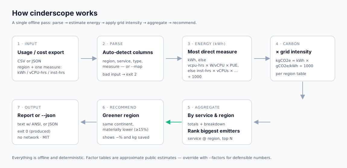
The whole thing is one deterministic pass. No model, no randomness, no API.

1. Parse and detect columns. Each row needs a region and one usage measure. Common column names (region, aws_region, location, machine_type, instance_hours, vcpu_hours, kwh, …) are auto-detected, ignoring case, spaces and underscores, so AWS Region and aws_region are the same thing. Anything unusual, you map explicitly:

cinderscope --map region=location,instance_type=sku,instance_hours=quantity bill.csv

2. Estimate energy (kWh) per row, using the most direct measure available:

energy(kWh) =
    kWh                                              if the export already measures it
    vcpu_hours × watts/vCPU × PUE / 1000             else
    instance_hours × vCPUs × watts/vCPU × PUE / 1000 else

If your export carries a measured kWh column, that wins - it's the most accurate input and skips the power model entirely. Otherwise cinderscope estimates server power from vCPU count (the approach the Cloud Carbon Footprint project popularised), using a per-family watt-per-vCPU figure. For the instance-hours path it even infers the vCPU count from the instance name across clouds - m5.2xlarge → 8, n2-standard-4 → 4, Standard_D4s_v5 → 4.

PUE (Power Usage Effectiveness) models datacenter overhead - cooling, power distribution - and defaults to 1.135. It's applied only to derived energy, never to a directly-measured kWh column, which is already end-to-end.

3. Apply grid intensity to get carbon.

carbon(kgCO2e) = energy(kWh) × region_intensity(gCO2e/kWh) / 1000

The unit dance matters and is easy to get wrong, so it's pinned by a test: 100 kWh in us-east-1 at 379 gCO2e/kWh must be exactly 100 × 379 / 1000 = 37.9 kgCO2e. Known input, known coefficient, known output.

4. Aggregate and rank by service and by region, and surface the top service @ region emitters.

5. Recommend a greener region. For each region you use, cinderscope looks for the lowest-intensity region on the same continent whose intensity is materially lower (at least 15%), and reports the percentage reduction and the kg you'd save by moving that load. Same-continent, because a recommendation that ignores latency and data residency is noise. It's a prompt to investigate, not an autopilot.

The honest part

I'd rather undersell this than have you quote it in an audit. So, plainly:

cinderscope produces a screening-level estimate, not an audited carbon figure. It's for ranking and prioritisation - finding the workload and the region that matter - not for regulatory reporting.

The reasons are baked into what "offline" costs you:

• The grid intensities are rounded, annual-average, point-in-time public figures, in the spirit of Cloud Carbon Footprint's coefficients and the Software Carbon Intensity methodology. They are not live, not marginal, and they will drift.

• Renewable purchasing is invisible to a grid average - a region where you buy 100% renewable PPAs still shows its grid number.

• It models operational electricity of compute only - not embodied/manufacturing carbon, not networking, not storage-at-rest.

• vCPU inference is a heuristic; a measured kwh or vcpu_hours column is always more accurate.

The right response to all of that is the --factors flag. You hand cinderscope a JSON file of your own coefficients - your provider's published intensities, your measured PUE, private on-prem regions - and it merges them onto the defaults. You only list what you want to change:

{
  "regions": {
    "us-east-1": { "intensity_gco2e_per_kwh": 350, "continent": "North America" },
    "my-onprem-1": { "intensity_gco2e_per_kwh": 480, "continent": "Europe" }
  },
  "family_watts_per_vcpu": { "m": 2.0, "r": 2.7 }
}

The defaults get you a directional answer in one command; --factors gets you a defensible one.

Where it fits

I keep a small family of tools that read the same billing/usage export and each answer one question well. cinderscope is deliberately the carbon one - separate from the dollar tools, because, as the Mumbai-vs-Paris example shows, carbon is a different ranking. It's a producer, not a gate: it emits a report and exits 0, or exits 2 on bad input. Wire the --json output into a dashboard, drop it in CI to watch a trend, or just run it on last month's export to see where your emissions actually are.

Try it

The code is MIT-licensed and on GitHub: github.com/jay-tank/cinderscope.

go install github.com/jay-tank/cinderscope@latest
cinderscope --json your-export.csv

Run it against a real export, then look at the biggest-emitter list next to your cost report. If the two rankings disagree - and they will - you've just found a carbon win the bill was hiding.